Purpose (TTS)

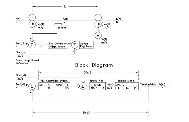
The Tension Through Speed (TTS) app is useful for checking the tuning and stability of a drive and controller working to hold tension in a web span. The system consists of two rollers driven by variable speed drives, the web in the span between the rollers, and a Proportional-Integral-Derivative (PID) controller adjusting the 2^nd drive’s speed to hold the measured tension to its setpoint.

This app may be used to enter the parameters for your system, and check tuning values for optimum tension control.

The model was inspired by research at Oklahoma State University [1]. A block diagram of the system is shown below.

Definitions

The tension model independent of the drive system may be studied using the TSpan app. TSpan shows the time constant and open loop gain of the web to a small step change in speed at the second roller. The time constant and open loop gain of the web tension to a speed change are important system parameters for initial tuning parameters in the tension regulator.

Parameters affected the tension model are:

Span (m) – distance between the driven rollers.

Gauge (mm) – thickness of the web

Width (m) – width of the web

Speed (m/min) – speed of the web.

Transfer Function – the relation between the output and input of a system. This is easily shown on a block diagram.

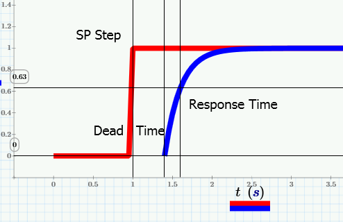
The Speed Regulator in the second drive introduces a lag equivalent to the speed regulator Bandwidth or Response or Gain (SRGN) in radians/second. This is the inverse of the speed regulator time constant if your drive refers to time constants. The time constant for a drive speed regulator is normally equal to the Speed Regulator Integral Gain (rad/sec) parameter in your drive. The response may be measured by providing a slack take up step to the drive and trending speed feedback. The time constant is the time (sec) for the speed feedback to reach 63% of its final value. The response is 1/ (time constant) (rad/sec).

The Parameter affection the tension model are:

The Modulus of Elasticity (E) is relates the strain of the web to the tension produced. E is measured in GPa or MPSI.

The PID controller has three parameters which may be used to tune the tension regulator. These are Proportional, Integral and Derivative. This app allows the user to change these parameters quickly to gain understanding of the system.

The PID controller is a classical controller. That is the classical control theory was developed in the 1930’s, but still has application today. Modern control theory was developed in the 1960’s to today and involves matrix solutions to the control problems. There are several methods of tuning the PID controller. These include:

1. Trial and Error algorithm. (Remember - engineering is a union of training and experience). Set Kd and Ki to zero. Set Kp to 1, step, review the response, halve or double Kp or the difference in Kp since the last step. Repeat for fastest response with no overshoot with Kp only. Reduce Kp to 60% of the value at the fastest response.
Set Ki to 1. Adjust Ki to 60% of the value with the fastest response.
Kd may not be required. In fact the regulator will be simpler and better behaved without Kd. Kd may be set and t60% of its optimum value found.
After Kd is set, it is often possible to raise Kp and Kd for better regulator response.

2. Tuning Algorithms such as Ziegler-Nichols.

3. Analytical methods which require a good model. Rules are used to determine the optimum gain settings mathematically and verify the results.

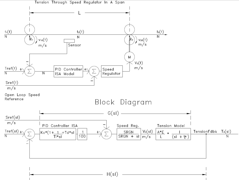
Two PID algorithms are available in industry and in this app. These are the Independent Model (iGain) and the ISA Model (Ideal Standard Algorithm – Wow what a mouthful). The ISA model is sometimes called the dependent model. Drive control engineers generally prefer the ISA model as it works with a single gain and two time constants. In the Independent model, changing any parameter affects two time constants. This app and most controllers support either PID model, but the default is often the Independent model. When tuned, both models produce identical results. However the method of tuning changes. Below is the block diagram showing the system with an ISA PID regulator.

The units used in the model are discussed later in this document.

Bode Plot

A classical technique using Bode plots which show system gain and phase shift vs. frequency are very useful in turning PID regulators. Rules have been developed which can be used to predict regulator response from the characteristics of the Bode Gain and Phase plots. We find that in order for a regulator to be stable with minimal overshoot, it should have a negative phase angle less than -135°. In practice, this is often between -90° and -135°. Additionally we see a stable regulator with minimal overshoot if the slope of the gain chart is -20 decibels (dB) per decade (frequency changes by a factor of 10) where the line crosses 0dB. The grid lines at 20dB and in decades on the Bode plot make it easy to determine the slope.

If the slope at the frequency where the line crosses 0dB (crossover frequency) is -20dB/decade, the phase at that crossover frequency is near -90°. Additionally the response of the regulator will be nearly equal to the crossover frequency in radians/second. The time constant of the regulator is the inverse of the crossover frequency.

Example 1:

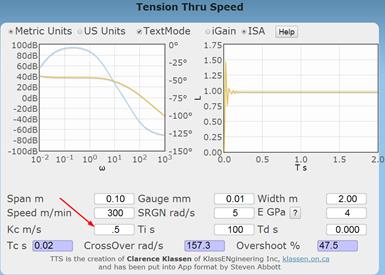
Set the parameters as shown. ISA Model, metric Kc=0.5 m/s, Ti=100 s (to get it out of the way), Td=0 sec. The speed regulator gain is 5.0 rad/sec. At this point the tuning is unsatisfactory showing overshoot, oscillations and not achieving the setpoint of 1 N. Adjust Kc to give a better response. Adjustments may increase or decrease the value. Note the slider in the app is cool, but in the real world each trial will take about 1 minute consuming web material for that entire minute. Therefore we generally halve or double the previous value or the difference to the previous value.

Hints for Tuning

Drive designers prefer the ISA model of the PID regulator. In order to tune the tension regulator through the speed regulator, it is useful to determine the model of web tension in the span. This can be determined with another Abbot App TSpan (Tension in a Span). TSpan provides a time constant for tension in this span when the speed of the second roller is given an incremental step change in speed. Run the TSpan app and enter the same parameters for the span and the web as are used in the TTS app.

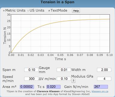
Record the time constant (0.02 seconds) calculated by TSpan. Switch back to TTS with the same parameters, ISA model and enter this time constant as Ti.

Set:
SRGN=5 radians/second (response of the 2^nd drive speed regulator)
Ti=Time Constant from TSpan
Td=0
G is adjusted to get a satisfying response. A satisfying response is exponential, has minimal overshoot and has a Crossover of 0.5 radians/second or higher.

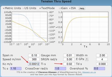
This is wonderful in that Ti and Td are preset and the response can be evaluated by adjusting a single parameter – G.

If the response shows overshoot, a value must be set into the Td parameter. I suggest entering 1/SRGN or 0.2 seconds.

I was able to achieve the following by adjusting Kc.

Notice that the crossover frequency read off the Bode plot is nearly identical to the response of the regulator shown on the time plot and shown as the CrossOver. You will notice the phase angle at the crossover frequency is between -90° and -135°.

“What If” Studies

Several of the model parameters may change over time. How will the tension regulator react to changing conditions. This is related to “robustness” of the control system.

Please note that regulator control is similar to warp speed and the Richter scale. Halving or doubling a parameter is about the minimum change that has a discernable effect on the regulator response.

The Modulus of Elasticity (E) is highly variable (factor of 3) depending on temperature, humidity and other physical conditions.

The Gauge is also highly variable and depends on your customer’s requirements.

The Span is difficult to change once the machine design is finalized. Experiment with longer and shorter spans.

The Speed Regulator Gain (SRGN) is dependent on the drive train and how well the drive is tuned. Defaults are from 5 to 10 radians/second for many new ac drives with rollers of modest inertia. High performance servo drives may achieve 100 radians/second. Note that Paper Machine drive speed regulators cannot be tuned for 5 radians/second.

Auto-tuning the drive provides a generic tuning value. Auto-tuning measures the inertia of the roller in units of seconds to reach full speed. The actual speed regulator gains are set based on this measured value. Most drives do not verify that the auto-tune results in the predicted speed regulator response. It is good to ask your drive tech to record a “step response” once tuning is complete. The step response should show the regulator response in radians/second and have no overshoot or ringing.

Theory - PID

The Proportional-Integral-Derivative (PID) regulator is well studied, as simple as can be, and suited for a wide variety of applications. The feedback filter is unity – that is tension feedback is not processed. The forward gain all acting on the tension error.

SetPoint (SP) – tension setpoint by the operator in N or lbs. In web handling we scale this to N/m or PLI.

Process Variable (PV) – measured tension feedback in N or lbs. In web handling we scale this to N/m or PLI.

Error (Err) = SP - PV

Control Variable (CV) – Output from the PID. In our case this is a speed increment with units of MPM or FPM.

Proportional Gain (Kp in Independent Model, G in ISA model) – the error is multiplied by this constant. Proportional gain alone cannot hold tension at its setpoint. The error cannot be reduced to zero.

Integral Gain (Ki in Independent Model, Ti in ISA model) – The error is integrated over time and multiplied by a constant. Integral control is required to regulate tension at the setpoint. The regulator must remember how much incremental speed is required to hold tension. Integration provides this memory.

Derivative Gain (Kd in Independent Model, Td in ISA model) – The error is differentiated or its rate of rise is determined and this is multiplied by a constant. Derivative is used to anticipate that the setpoint is being achieved and reduces the change in CV.

The time constants in the Independent Model PID change when any of Kp, Ki or Kd are changed. Often it is necessary to change all 3 gains together to keep time constants correct.

The ISA Model PID keeps the two time constants constant when changing the gain. We use:

G – Gain of the regulator (identical to Kp in the Independent Model)

Ti – Time constant corresponding to the integral action. It is not possible to set Ti=0 so the ISA model supports a PI or PID regulator, but not a P only regulator.

Td – Time constant corresponding to the derivative action. This may be set to zero to produce a PI regulator.

Drive engineers prefer the ISA Model because we can measure or calculate physical time constants in the plant and cancel them with Ti and Td in the PID regulator. For example, I suggest using the TSpan app to calculate the time constant of tension in the web. Put this value into Ti. Then put the time constant of the drive speed regulator (1/SRGN) into Td. With Ti and Td preset, there is only one parameter (G) needed to tune the tension regulator.

Of course the guidance above does not prevent you from learning while playing with the TTS app.

Note: Very little speed change is required to achieve tension. Therefore the output of the PID tension regulator is divided by 100 as shown in the block diagram.

Units

Units of measurement are as important as values of measurements. Units are consistent in the TTS app. Refer to the block diagram starting at the Right Hand side and working to the left.

The final desired output is the tension force. The model shows this force in Newtons (N). The web handling industry prefers to normalize tension into PLI or N/m, however the model used is in units of N.

Tension is created by a draw % or increment in speed between two rollers with traction. The speed difference is measured in m/sec or ft./sec. The tension model (detailed in the TSpan app) used in the TTS app converts the m/sec difference to a tension force in N.

The simplified speed regulator block is itself a closed loop regulator (PID or more complex) plus an ac motor vector controller with a model of the motor and roller. The simplified model of the speed regulator represents a simple model after the drive tech has performed auto-tune on the drive. The drive tech has verified the auto-tune and verified the response of the speed regulator is exponential with no overshoot or oscillations.

The PV for the speed regulator is motor RPM scaled by the roller circumference and gear ratio to m/sec. The output of the speed regulator is also in m/sec. Thus the speed regulator does not change units – m/sec in and m/sec out.

The PID tension regulator PV has units of force (N). The output of the tension regulator is in m/sec. Thus the PID regulator converts units of force (N) into units of speed (m/sec).

Each of the PID regulator gains perform the same conversion. Note that the PID regulator is general purpose and the units are scaled to % in the documentation. The PID regulator may be used with temperature, level, pressure, colour, gauge, position, …, even tension). So the units displayed in the tuning software and described in the help are normalized to %out over %in.

Gain in TTS	Units Described in the PID
Independent Model
Kp * N = m/sec Kp = m / sec / N	%out / %in
Ki/1/sec * N = m/sec Ki = m / sec^2 / N	%out / sec / %in
Kd/sec * N = m/sec Kd = m / N	%out * sec / %in
ISA Model
G * N = m/sec G = m / sec / N	%out / %in
Ti/sec * N = m/sec Ti = m / N	%out / sec / %in
Td*sec * N = m/sec Td = m / sec^2 / N	%out * sec / %in

Bode Plots – Theory

Bode Plots are used in classical control theory to simplify and analyse the complexity of control theory. Bode plots have been used since the 1930’s and are still used today to supplement modern control theory methods.

Control theory involves the solution of simultaneous differential equations. Furthermore the forcing function for the differential equations is typically discontinuous (ex. stopped, ramp to speed, hold speed, accelerate some more, decelerate, stop).

It turns out that Laplace domain methods have a number of advantages for the analysis of control system equations. These are:

- The Laplace transform starts with the initial conditions. No history before the initial conditions is assumed or required.

- Cascading of transfer functions is simple multiplication in the Laplace domain.

- Time shifts in the forcing function are simply accomplished.

The major downside of Laplace domain methods is in performing the inverse Laplace transform to get a chart of the regulator response in the time domain.

The Bode Plot was developed to plot the complex transfer functions as parametric equations in gain and phase vs. frequency. Gain of a function is plotted on a log scale (actually decibels or dB) vs frequency also on a log scale. Phase shift is plotted on a linear scale vs. frequency on a log scale.

The function plotted is a “part of the closed loop” regulator function called the “open loop” regulator function. When shown on the Bode plot, the “open loop” function can be used to predict the result of the “closed loop” function.

If the forward gain of the function is represented by G and the feedback function is represented by H, we use the closed loop function to simplify the transfer function of the system. The transfer function in the Laplace domain becomes:

G/(1+G*H)           picture here

Study and experience have shown that the most interesting features of transfer functions occur when the denominator is near zero. In modern control theory further simplifications are performed to determine the exact polynomial form of the denominator or characteristic equation.

The denominator 1 + G*H is not exactly, but may be compared with the characteristic equation of modern control theory.

So we are interested in the denominator when it is equal to zero.

1 + G*H = 0

G*H = 1 = 0 dB

Bode Plots – Used for Tuning

The Bode plot shows the gain and phase vs. frequency. It is easy to read the frequency at which the gain is 0dB. We call this the crossover frequency. We can easily read the slope of the gain curve and the phase angle at that frequency.

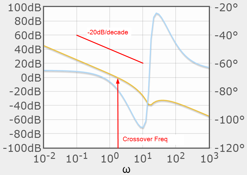
The PID gain parameters may be modified to change the slope of the gain plot and adjust the phase shift at the crossover frequency. Stable regulators, as designed using classical control theory, follow a few rules.

1. The gain plot should cross the 0dB line at only once.

2. The slope of the gain plot should be -20dB/decade at the crossover frequency

3. The phase shift at the crossover frequency should be between -90° and -135°. If the slope of the gain plot is -20dB/decade, this requirement is met.

4. The crossover determines the bandwidth or response of the regulator.

5. The phase shift determines the overshoot. At -90° there is no overshoot.

6. Increasing the regulator gain will improve the response of the regulator until one of the rules is violated.

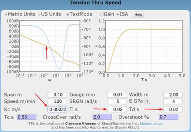
So to tune the tension regulator in the TTS app

1. Use the ISA model

2. Run TSpan app to determine the time constant for the web in a span. Enter this in Ti.

3. Set Td = 0

4. Set the gain G to get the crossover to 1 radian/second.

5. Check the slope of the gain plot between 0.1 and 10 rad/sec. It should be about -20dB/decade.

6. If not, enter the inverse of speed regulator gain into Td.

7. The Bode plot gain should have a slope of -20dB/decade at the crossover of 1 radian/second.

8. Check the phase plot. It should be between -90° and -135° at 1 the crossover frequency.

9. Check the tension regulator response. We are looking for an exponential with no overshoot. The time constant is equal to 1/crossover = 1 second.

10. Adjust the Ti and Td to get the best looking response with a 1 second time constant. Try this by adjusting G first.

Observations by the Author

The TTS app results in regulator gains approximately 10 times smaller than actual tuned values in the field. I have checked the math several different ways with the same results. This may indicate:

1. I have implemented the tension model or the PID model incorrectly.

2. The modulus of Elasticity is much lower than predicted while material is being produce on actual lines due to temperature and other physical effects.

3. The rollers are slipping on the web.

I welcome any comments from those using this app.

Sample Code (Matlab™)

The TTS app is written in Java script. Below is equivalent Matlab code.

## Author: cjk Tension Through Speed 2014Feb15

more off # stop showing intermediate results

L=0.1 ## m

G=0.05E-3 ## m

W=2.0 ## m

V=5.0 ## m/sec

SRGN=5.0 ## rad/sec

E=1.2E9 ## Pa

AUTH=1.0 ## %

## Independent Model

Kp=0.001 ## m/sec

Ki=0.01 ## m/sec^2

Kd=0.0 ## m

A=G*W

PIDnum = AUTH/100*[Kd Kp Ki]

PIDden = [1 0]

SRnum = SRGN

SRden = [1 SRGN]

Tnum = A*E/L ## set up the Tension transfer function

Tden = [1 V/L]

## set up the numerator and denominator for the open loop transfer function. Combine the PID, Plant and tension Model.

Golnum1 = conv(conv (PIDnum, SRnum), Tnum)

Golden1 = conv(conv (PIDden, SRden), Tden)

Gol = tf(Golnum1, Golden1) ## Combine the numerator and denominator to form the open loop gain

## The tension model forms the feedback for the closed loop system

Hol = [1]

## Determine the closed loop response of the system (cloop in Matlab)

Gcl = feedback (Gol, Hol)

step (Gcl,5)

Comments on the model:

· We assume the first roller is the line master and is driven at and holds line speed exactly.

· There is no noise or filtering on the measured tension feedback

· The Speed Regulator Time Constant in the tension controlling drive is considered.

References

[1] Tension Control Kee-Hyun Shin, Tappi Press, 2000, ISNB 0-89852-348-6,